Theory
Before the system can be modelled in ESL the fundamental governing equations must be derived. This can be done by considering the interaction between the thermodynamic and dynamic properties of the system.
Defining Constants and Variables

Part-Section of the Engine
First, the symbols used to define all the constants and variables must be understood.
---Definitions to go here:
---Definitions to go here:
From the diagram above, the position of the displacer piston can be represented by equation 1.
Similarly, the position of the working (power) piston is shown in equation 2.
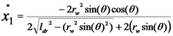
These displacement equations can be derived with respect to the relative crank angle to give velocity. The expression for x1 is given in equation 3.
The expression for x2 is given in equation 4.
The volume of the hot end of the displacer cylinder at any point depends on the position of the displacer piston as well as the clearance volume and is given in equation 5.
If this is differentiated with respect to x1 we are left with this equation:
For the cold side of the system, as before, the clearance volumes must be taken into account but this time the volume of the working piston must be considered also.
Again, this was differentiated with respect to x1 and x2 to give equation 8.
The crank angles can be calculated using basic trigonometry. Equations 9 and 10 show the angle of the displacer piston and power piston crank angles respectively.
Similarly, the angle between the crankwheel tangent and crank angle can be calculated using trigonometric functions. Equations 11 and 12 show this angle for the displacer piston and power piston respectively.
The Ideal Gas Law can be applied to both the hot and cold ends of the displacer piston as shown in equations 13 and 14.
Using the Ideal Gas Law again, this time in its partial derivative form, the air flow around the displacer piston can be represented by equation 15.
Equation 16 donates the differential of equation 15 with respect to time.
Now substituting in equation 6 to give equation 17.
This is part of a polytropic process which can be represented by equation 18.
Equation 18 is then differentiated with respect to time and, as before, equation 6 is substituted in to result in equation 19.
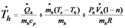
Considering the hot end of the displacer cylinder: by rearranging equation 17 to be in terms of rate of change of time, substituting in equation 19, and taking into account the addition of heat energy, we are left with equation 20.
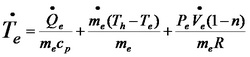
The equation for the rate of heat addition for the cold end of the cylinder can be derived in a similar way. It is shown in equation 21.
Before the expressions for the heat in and heat out can be formulated, the areas upon which they act must be calculated. This is shown for the hot side (heat addition) in equation 22.
For the heat rejection at the cold side of the cylinder, the area is denoted by equation 23.
The heat energy which is added to the cylinder is given in equation 24.
The heat energy removed by the cold cap is given in equation 25.
The force of the displacer piston can be found by taking the difference between the pressure on the hot and cold areas of the ends of the displacer cylinder. This is shown in equation 26.
Likewise, the force of the work piston can be found by taking the difference between the pressure on the cooled face of the piston and the pressure of the piston on the atmosphere. This is shown in equation 27.
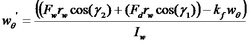
finally, the rotational velocity of the flywheel can be found using equation 28. This can be used in conjunction with other variables to plot various results.
Similarly, the position of the working (power) piston is shown in equation 2.
These displacement equations can be derived with respect to the relative crank angle to give velocity. The expression for x1 is given in equation 3.
The expression for x2 is given in equation 4.
The volume of the hot end of the displacer cylinder at any point depends on the position of the displacer piston as well as the clearance volume and is given in equation 5.
If this is differentiated with respect to x1 we are left with this equation:
For the cold side of the system, as before, the clearance volumes must be taken into account but this time the volume of the working piston must be considered also.
Again, this was differentiated with respect to x1 and x2 to give equation 8.
The crank angles can be calculated using basic trigonometry. Equations 9 and 10 show the angle of the displacer piston and power piston crank angles respectively.
Similarly, the angle between the crankwheel tangent and crank angle can be calculated using trigonometric functions. Equations 11 and 12 show this angle for the displacer piston and power piston respectively.
The Ideal Gas Law can be applied to both the hot and cold ends of the displacer piston as shown in equations 13 and 14.
Using the Ideal Gas Law again, this time in its partial derivative form, the air flow around the displacer piston can be represented by equation 15.
Equation 16 donates the differential of equation 15 with respect to time.
Now substituting in equation 6 to give equation 17.
This is part of a polytropic process which can be represented by equation 18.
Equation 18 is then differentiated with respect to time and, as before, equation 6 is substituted in to result in equation 19.
Considering the hot end of the displacer cylinder: by rearranging equation 17 to be in terms of rate of change of time, substituting in equation 19, and taking into account the addition of heat energy, we are left with equation 20.
The equation for the rate of heat addition for the cold end of the cylinder can be derived in a similar way. It is shown in equation 21.
Before the expressions for the heat in and heat out can be formulated, the areas upon which they act must be calculated. This is shown for the hot side (heat addition) in equation 22.
For the heat rejection at the cold side of the cylinder, the area is denoted by equation 23.
The heat energy which is added to the cylinder is given in equation 24.
The heat energy removed by the cold cap is given in equation 25.
The force of the displacer piston can be found by taking the difference between the pressure on the hot and cold areas of the ends of the displacer cylinder. This is shown in equation 26.
Likewise, the force of the work piston can be found by taking the difference between the pressure on the cooled face of the piston and the pressure of the piston on the atmosphere. This is shown in equation 27.
finally, the rotational velocity of the flywheel can be found using equation 28. This can be used in conjunction with other variables to plot various results.

Equation 1

Equation 2
Equation 3

Equation 4

Equation 5

Equation 6

Equation 7

Equation 8

Equation 9

Equation 10

Equation 11

Equation 12

Equation 13

Equation 14

Equation 15

Equation 16

Equation 17

Equation 18

Equation 19
Equation 20
Equation 21

Equation 22

Equation 23

Equation 24

Equation 25

Equation 26

Equation 27
Equation 28
Once these equations had been derived, they were input into a sequential order into an ESL file. The constant were also defined as well as the desired output information. A variety of different information can be obtained from the ESL software which allowed us to analyse the theoretical performance of our engine design and can be found in the ESL Results section. The complete log file can be viewed in the file below.
| esl_log_file.txt |
